

How To Draw The Derivative Of A Rational Function
four. Applications of Derivatives
four.6 Limits at Infinity and Asymptotes
Learning Objectives
We have shown how to apply the offset and second derivatives of a function to describe the shape of a graph. To graph a role  defined on an unbounded domain, we also demand to know the beliefs of as
  In this department, we define limits at infinity and bear witness how these limits affect the graph of a part. At the finish of this section, nosotros outline a strategy for graphing an arbitrary function
Limits at Infinity
We begin by examining what it means for a role to take a finite limit at infinity. And so we study the idea of a function with an space limit at infinity. Back in Introduction to Functions and Graphs, we looked at vertical asymptotes; in this section nosotros deal with horizontal and oblique asymptotes.
Limits at Infinity and Horizontal Asymptotes
Call back that  ways
ways  becomes arbitrarily close to
  as long as
  is sufficiently close to
  We tin can extend this thought to limits at infinity. For instance, consider the role
  As tin can be seen graphically in (Figure) and numerically in (Figure), as the values of go larger, the values of approach two. Nosotros say the limit as approaches
  of is two and write
  Similarly, for
  as the values
  get larger, the values of approaches 2. We say the limit equally approaches
  of is 2 and write
| | 10 | 100 | 1,000 | 10,000 |
 | 2.i | 2.01 | 2.001 | 2.0001 |
| | -x | -100 | -1000 | -10,000 |
| | 1.9 | 1.99 | ane.999 | 1.9999 |
More by and large, for any function  we say the limit as
  of is if becomes arbitrarily close to as long every bit is sufficiently big. In that case, we write
  Similarly, we say the limit equally
  of is if becomes arbitrarily close to as long equally
  and is sufficiently large. In that example, we write
  We now look at the definition of a part having a limit at infinity.
If the values are getting arbitrarily close to some finite value equally or  the graph of approaches the line
  In that case, the line
  is a horizontal asymptote of ((Figure)). For example, for the function
  since
since  the line
  is a horizontal asymptote of
Definition
If  or
or  nosotros say the line is a horizontal asymptote of
A role cannot cross a vertical asymptote because the graph must arroyo infinity (or  from at least one direction as approaches the vertical asymptote. However, a function may cross a horizontal asymptote. In fact, a role may cantankerous a horizontal asymptote an unlimited number of times. For case, the function
  shown in (Effigy) intersects the horizontal asymptote
  an space number of times as it oscillates around the asymptote with e'er-decreasing amplitude.
The algebraic limit laws and clasp theorem we introduced in Introduction to Limits likewise apply to limits at infinity. We illustrate how to utilize these laws to compute several limits at infinity.
Computing Limits at Infinity
Solution
- Using the algebraic limit laws, we have
 Similarly,
  Therefore,
  has a horizontal asymptote of
  and approaches this horizontal asymptote equally
  equally shown in the following graph.
 - Since
 for all
  we have
for all
 Also, since
we tin can utilize the squeeze theorem to conclude that

Similarly,

Thus,
 has a horizontal asymptote of and approaches this horizontal asymptote as as shown in the following graph.
Figure 5. This part crosses its horizontal asymptote multiple times. - To evaluate
 and
and  we beginning consider the graph of
  over the interval
  equally shown in the post-obit graph.
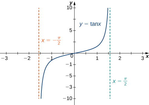
The graph of
 has vertical asymptotes at
Since

it follows that

Similarly, since

it follows that

As a result,  and
and  are horizontal asymptotes of
  as shown in the following graph.
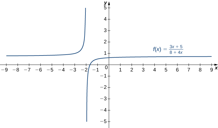
Evaluate  and
and  Determine the horizontal asymptotes of
  if whatsoever.
Solution
Both limits are 3. The line  is a horizontal asymptote.
Infinite Limits at Infinity
Sometimes the values of a part get arbitrarily large as (or equally  In this case, we write
  (or
(or  On the other paw, if the values of are negative only get arbitrarily large in magnitude every bit (or as
  we write
  (or
(or 
For example, consider the function  As seen in (Figure) and (Figure), every bit the values become arbitrarily large. Therefore,
  On the other mitt, as the values of
  are negative but get arbitrarily large in magnitude. Consequently,
| | 10 | 20 | 50 | 100 | yard |
 | 1000 | 8000 | 125,000 | 1,000,000 | 1,000,000,000 |
| | -10 | -20 | -fifty | -100 | -1000 |
| | -thou | -8000 | -125,000 | -1,000,000 | -1,000,000,000 |
Definition
(Informal) Nosotros say a function has an infinite limit at infinity and write

if becomes arbitrarily large for sufficiently large. We say a office has a negative infinite limit at infinity and write

if  and
and  becomes arbitrarily big for sufficiently big. Similarly, we can define infinite limits as
Formal Definitions
Before, nosotros used the terms arbitrarily close, arbitrarily large, and sufficiently big to ascertain limits at infinity informally. Although these terms provide accurate descriptions of limits at infinity, they are not precise mathematically. Here are more formal definitions of limits at infinity. We then look at how to use these definitions to show results involving limits at infinity.
Definition
(Formal) We say a part has a limit at infinity, if there exists a existent number such that for all  there exists
  such that

for all  In that instance, we write
(see (Figure)).
Nosotros say a function has a limit at negative infinity if there exists a real number such that for all in that location exists  such that
for all  In that case, we write
Earlier in this section, we used graphical evidence in (Figure) and numerical evidence in (Figure) to conclude that  Here we use the formal definition of limit at infinity to prove this upshot rigorously.
A Finite Limit at Infinity Example
Use the formal definition of limit at infinity to prove that
Solution
Allow  Let
Let  Therefore, for all
  we have

Apply the formal definition of limit at infinity to prove that 
Solution
Permit Let  Therefore, for all we accept

Therefore, 
Nosotros now turn our attention to a more precise definition for an space limit at infinity.
Definition
(Formal) We say a role has an space limit at infinity and write
if for all  there exists an such that

for all  (see (Figure)).
Nosotros say a part has a negative space limit at infinity and write
if for all  there exists an such that

for all
Similarly we tin define limits as
Earlier, we used graphical evidence ((Figure)) and numerical evidence ((Effigy)) to conclude that Here we use the formal definition of space limit at infinity to testify that result.
An Space Limit at Infinity
Use the formal definition of infinite limit at infinity to prove that
Solution
Let  Allow
Allow ![N=\sqrt[3]{M}.](https://opentextbc.ca/calculusv1openstax/wp-content/ql-cache/quicklatex.com-5d31222eb8da1be538b8274beb5a60e8_l3.png "Rendered by QuickLaTeX.com") Then, for all we have
Then, for all we have
![{x}^{3}>{N}^{3}={(\sqrt[3]{M})}^{3}=M.](https://opentextbc.ca/calculusv1openstax/wp-content/ql-cache/quicklatex.com-7885f71d42b2b93e5cd5500320c1d0fa_l3.png "Rendered by QuickLaTeX.com")
Therefore,
Utilize the formal definition of space limit at infinity to evidence that 
Solution
Let Allow  Then, for all we have

End Beliefs
The beliefs of a office every bit is called the function's end beliefs. At each of the function's ends, the function could exhibit one of the following types of behavior:
- The role approaches a horizontal asymptote
- The function
 or
or 
- The function does not arroyo a finite limit, nor does information technology approach or
 In this instance, the function may have some oscillatory behavior.
Let's consider several classes of functions hither and look at the dissimilar types of terminate behaviors for these functions.
End Behavior for Polynomial Functions
Consider the power role  where
where  is a positive integer. From (Effigy) and (Figure), we meet that

and

Using these facts, it is non difficult to evaluate  and
and  where
where  is whatsoever constant and is a positive integer. If
  the graph of
  is a vertical stretch or compression of
  and therefore

If  the graph of is a vertical stretch or compression combined with a reflection about the -axis, and therefore

If  in which case
Limits at Infinity for Power Functions
We now look at how the limits at infinity for power functions can be used to make up one's mind  for any polynomial function Consider a polynomial function

of degree  and then that
  Factoring, we see that

Equally  all the terms inside the parentheses approach zero except the first term. Nosotros conclude that

For case, the function  behaves like
  every bit as shown in (Figure) and (Effigy).

| | 10 | 100 | thousand |
| | 4704 | 4,970,004 | 4,997,000,004 |
| | 5000 | 5,000,000 | 5,000,000,000 |
| | -10 | -100 | -thousand |
| | -5296 | -5,029,996 | -5,002,999,996 |
| | -5000 | -5,000,000 | -5,000,000,000 |
Terminate Behavior for Algebraic Functions
The end behavior for rational functions and functions involving radicals is a little more complicated than for polynomials. In (Figure), we show that the limits at infinity of a rational office  depend on the human relationship between the caste of the numerator and the caste of the denominator. To evaluate the limits at infinity for a rational function, nosotros divide the numerator and denominator by the highest power of appearing in the denominator. This determines which term in the overall expression dominates the behavior of the office at large values of
Determining Stop Behavior for Rational Functions
Evaluate  and use these limits to determine the cease behavior of
Solution

Earlier proceeding, consider the graph of  shown in (Effigy). As and the graph of appears almost linear. Although is certainly not a linear function, we at present investigate why the graph of seems to exist approaching a linear function. First, using long sectionalization of polynomials, nosotros tin write

Since  as we conclude that

Therefore, the graph of approaches the line  equally This line is known every bit an oblique asymptote for ((Figure)).
Nosotros can summarize the results of (Figure) to make the following conclusion regarding end behavior for rational functions. Consider a rational function

where 
- If the caste of the numerator is the same as the degree of the denominator
 then has a horizontal asymptote of
  every bit
 - If the degree of the numerator is less than the degree of the denominator
 so has a horizontal asymptote of as
 - If the caste of the numerator is greater than the degree of the denominator
 then does non have a horizontal asymptote. The limits at infinity are either positive or negative infinity, depending on the signs of the leading terms. In addition, using long division, the function can be rewritten equally
where the caste of
 is less than the caste of
  As a effect,
  Therefore, the values of
 ![\left[f(x)-g(x)\right]](https://opentextbc.ca/calculusv1openstax/wp-content/ql-cache/quicklatex.com-d74b22dc7ee32570ba55c128113aec8f_l3.png "Rendered by QuickLaTeX.com") approach zero as If the degree of
approach zero as If the degree of  is exactly one more than the degree of
 the function
  is a linear function. In this case, nosotros telephone call an oblique asymptote.
Now let'due south consider the cease beliefs for functions involving a radical.
Determining Finish Behavior for a Function Involving a Radical
Evaluate 
Solution

Guidelines for Drawing the Graph of a Function
We now have enough belittling tools to draw graphs of a wide variety of algebraic and transcendental functions. Before showing how to graph specific functions, let's look at a general strategy to employ when graphing any function.
At present allow's use this strategy to graph several different functions. Nosotros first past graphing a polynomial function.
Sketching a Graph of a Polynomial
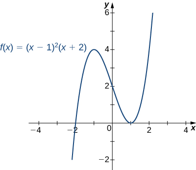
Sketch a graph of 
Solution
Step 1. Since is a polynomial, the domain is the set of all existent numbers.
Stride ii. When  Therefore, the
  -intercept is
  To find the -intercepts, nosotros need to solve the equation
  gives united states of america the -intercepts
  and
and 
Step 3. We need to evaluate the terminate beliefs of As 
 and
and  Therefore, Every bit and
  Therefore, To become even more than information about the stop behavior of we can multiply the factors of When doing and so, nosotros see that

Since the leading term of is  we conclude that behaves similar
  as
as
Step 4. Since is a polynomial function, it does not accept whatever vertical asymptotes.
Step five. The starting time derivative of is

Therefore, has two disquisitional points:  Divide the interval
  into the three smaller intervals:
 and
and  So, choose test points
 and
and  from these intervals and evaluate the sign of
  at each of these test points, as shown in the following tabular array.
| Interval | Exam Point | Sign of Derivative  | Conclusion |
|---|---|---|---|
 |  |  | is increasing. |
 |  |  | is decreasing. |
 | |  | is increasing. |
From the table, nosotros see that has a local maximum at  and a local minimum at
  Evaluating at those two points, nosotros notice that the local maximum value is
  and the local minimum value is
Step 6. The second derivative of is

The second derivative is zero at  Therefore, to make up one's mind the concavity of divide the interval into the smaller intervals
  and
and  and choose examination points and
  to determine the concavity of on each of these smaller intervals as shown in the following tabular array.
| Interval | Test Bespeak | Sign of  | Conclusion |
|---|---|---|---|
| | |  | is concave downwards. |
 | |  | is concave up. |
We notation that the information in the preceding table confirms the fact, establish in step v, that has a local maximum at and a local minimum at In add-on, the information found in step 5—namely, has a local maximum at and a local minimum at  and
and  at those points—combined with the fact that
  changes sign only at confirms the results establish in step 6 on the concavity of
Combining this information, we arrive at the graph of  shown in the following graph.
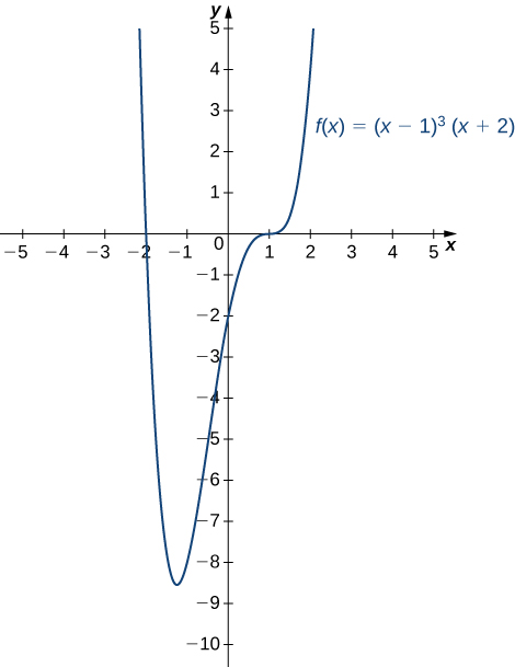
Sketch a graph of 
Solution
Sketching a Rational Office
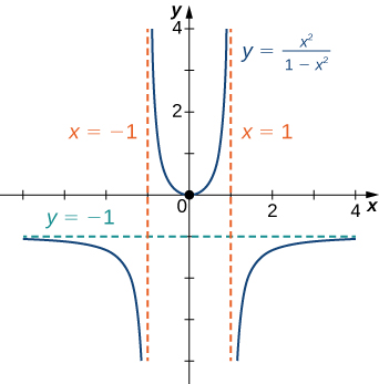
Sketch the graph of 
Solution
Step 1. The function is defined equally long as the denominator is not naught. Therefore, the domain is the set of all real numbers except 
Step 2. Detect the intercepts. If and so  so 0 is an intercept. If
  and so
  which implies Therefore,
  is the merely intercept.
Step 3. Evaluate the limits at infinity. Since is a rational part, divide the numerator and denominator by the highest power in the denominator:  We obtain

Therefore, has a horizontal asymptote of  as and
Step 4. To determine whether has any vertical asymptotes, first cheque to see whether the denominator has any zeroes. We find the denominator is zero when To decide whether the lines or are vertical asymptotes of evaluate  and
and  By looking at each one-sided limit every bit
  we run into that

In addition, by looking at each one-sided limit as  we find that

Step 5. Calculate the commencement derivative:

Critical points occur at points where or is undefined. We see that when The derivative  is not undefined at any bespeak in the domain of However,
  are not in the domain of Therefore, to make up one's mind where is increasing and where is decreasing, divide the interval into four smaller intervals:
 and
and  and cull a examination point in each interval to decide the sign of in each of these intervals. The values
 and are good choices for test points equally shown in the following table.
| Interval | Examination Indicate | Sign of  | Conclusion |
|---|---|---|---|
| | |  | is decreasing. |
 |  | | is decreasing. |
 |  |  | is increasing. |
| | | | is increasing. |
From this analysis, nosotros conclude that has a local minimum at simply no local maximum.
Step six. Calculate the second derivative:
![\begin{array}{cc}\hfill f\text{″}(x)& \hfill =\frac{{(1-{x}^{2})}^{2}(2)-2x(2(1-{x}^{2})(-2x))}{{(1-{x}^{2})}^{4}}\\ & =\frac{(1-{x}^{2})\left[2(1-{x}^{2})+8{x}^{2}\right]}{{(1-{x}^{2})}^{4}}\hfill \\ & =\frac{2(1-{x}^{2})+8{x}^{2}}{{(1-{x}^{2})}^{3}}\hfill \\ & =\frac{6{x}^{2}+2}{{(1-{x}^{2})}^{3}}.\hfill \end{array}](https://opentextbc.ca/calculusv1openstax/wp-content/ql-cache/quicklatex.com-3c88196c67780e8cb98b05116b8e263a_l3.png "Rendered by QuickLaTeX.com")
To determine the intervals where is concave up and where is concave downward, we starting time need to find all points where  or
or  is undefined. Since the numerator
  for any is never zero. Furthermore, is non undefined for any in the domain of However, as discussed earlier, are not in the domain of Therefore, to make up one's mind the concavity of we divide the interval into the three smaller intervals
  and and choose a examination point in each of these intervals to evaluate the sign of
  in each of these intervals. The values and are possible test points as shown in the post-obit table.
| Interval | Examination Point | Sign of  | Conclusion |
|---|---|---|---|
| | |  | is concave down. |
 | | | is concave upwards. |
| | | | is concave downwardly. |
Combining all this information, we arrive at the graph of shown beneath. Notation that, although changes concavity at and there are no inflection points at either of these places because is not continuous at or
Sketch a graph of 
Solution
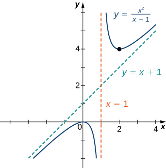
Sketching a Rational Function with an Oblique Asymptote
Sketch the graph of 
Solution
Step 1. The domain of is the set of all real numbers except
Footstep ii. Find the intercepts. We tin run into that when so is the only intercept.
Pace three. Evaluate the limits at infinity. Since the degree of the numerator is 1 more than the caste of the denominator, must take an oblique asymptote. To notice the oblique asymptote, use long division of polynomials to write

Since  every bit approaches the line
  every bit The line is an oblique asymptote for
Step 4. To cheque for vertical asymptotes, wait at where the denominator is zippo. Here the denominator is zero at Looking at both one-sided limits as nosotros find

Therefore, is a vertical asymptote, and we accept adamant the behavior of every bit approaches 1 from the right and the left.
Step 5. Calculate the first derivative:

Nosotros have when  Therefore, and are disquisitional points. Since is undefined at we need to divide the interval into the smaller intervals
 and
and  and cull a examination point from each interval to evaluate the sign of in each of these smaller intervals. For example, let
 and
and  be the test points as shown in the following table.
| Interval | Test Point | Sign of  | Determination |
|---|---|---|---|
| | |  | is increasing. |
| | |  | is decreasing. |
 |  | | is decreasing. |
 | |  | is increasing. |
From this tabular array, we see that has a local maximum at and a local minimum at  The value of at the local maximum is
  and the value of at the local minimum is
  Therefore, and
  are important points on the graph.
Step half dozen. Calculate the 2d derivative:
![\begin{array}{cc}\hfill f\text{″}(x)& =\frac{{(x-1)}^{2}(2x-2)-({x}^{2}-2x)(2(x-1))}{{(x-1)}^{4}}\hfill \\ & =\frac{(x-1)\left[(x-1)(2x-2)-2({x}^{2}-2x)\right]}{{(x-1)}^{4}}\hfill \\ & =\frac{(x-1)(2x-2)-2({x}^{2}-2x)}{{(x-1)}^{3}}\hfill \\ & =\frac{2{x}^{2}-4x+2-(2{x}^{2}-4x)}{{(x-1)}^{3}}\hfill \\ & =\frac{2}{{(x-1)}^{3}}.\hfill \end{array}](https://opentextbc.ca/calculusv1openstax/wp-content/ql-cache/quicklatex.com-f884d8d96e071a11fbe634b87f16b6ea_l3.png "Rendered by QuickLaTeX.com")
We meet that is never zilch or undefined for in the domain of Since is undefined at to check concavity nosotros just divide the interval into the ii smaller intervals  and and choose a examination point from each interval to evaluate the sign of in each of these intervals. The values and are possible examination points as shown in the post-obit table.
| Interval | Exam Point | Sign of  | Conclusion |
|---|---|---|---|
| | | | is concave downward. |
| | | | is concave upwardly. |
From the information gathered, we arrive at the following graph for
Find the oblique asymptote for 
Solution

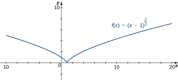
Sketching the Graph of a Function with a Cusp
Sketch a graph of 
Solution
Step one. Since the cube-root office is defined for all existent numbers and ![{(x-1)}^{2\text{/}3}={(\sqrt[3]{x-1})}^{2},](https://opentextbc.ca/calculusv1openstax/wp-content/ql-cache/quicklatex.com-b1c1401791ff1f2c6e3594979b4a0681_l3.png "Rendered by QuickLaTeX.com") the domain of is all real numbers.
the domain of is all real numbers.
Step ii: To find the -intercept, evaluate  Since
Since  the -intercept is
  To find the -intercept, solve
  The solution of this equation is and then the -intercept is
Pace 3: Since  the function continues to abound without bound equally and
Footstep four: The function has no vertical asymptotes.
Step 5: To make up one's mind where is increasing or decreasing, calculate  Nosotros find

This function is not zero anywhere, just it is undefined when Therefore, the merely critical point is Divide the interval into the smaller intervals and and choose exam points in each of these intervals to determine the sign of in each of these smaller intervals. Let and exist the exam points every bit shown in the post-obit tabular array.
| Interval | Test Signal | Sign of  | Conclusion |
|---|---|---|---|
| | | | is decreasing. |
| | | | is increasing. |
Nosotros conclude that has a local minimum at Evaluating at we find that the value of at the local minimum is zero. Annotation that  is undefined, so to determine the behavior of the part at this critical point, we need to examine
  Looking at the ane-sided limits, we have

Therefore, has a cusp at
Pace 6: To determine concavity, nosotros calculate the 2d derivative of 

Nosotros detect that is defined for all just is undefined when Therefore, divide the interval into the smaller intervals and and cull test points to evaluate the sign of in each of these intervals. As we did earlier, let and exist test points as shown in the following tabular array.
| Interval | Test Point | Sign of  | Conclusion |
|---|---|---|---|
| | | | is concave downwardly. |
| | | | is concave downwards. |
From this table, nosotros conclude that is concave downward everywhere. Combining all of this information, we arrive at the following graph for
Consider the role  Make up one's mind the point on the graph where a cusp is located. Determine the finish behavior of
Primal Concepts
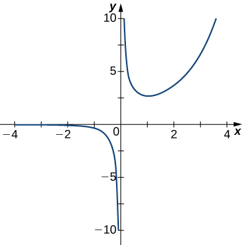
For the following exercises, examine the graphs. Identify where the vertical asymptotes are located.
1. 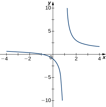
Solution
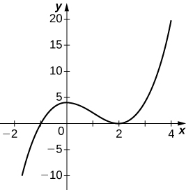
2. 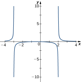
3. 
Solution

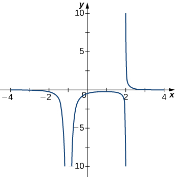
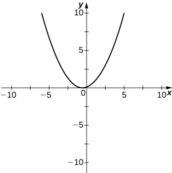
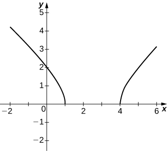
iv.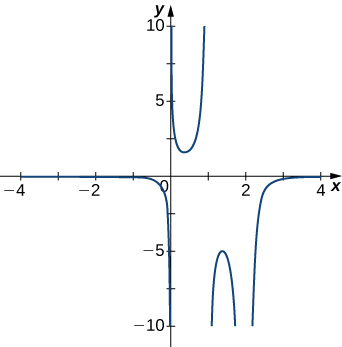
5.
Solution
For the following functions  make up one's mind whether there is an asymptote at
  Justify your answer without graphing on a calculator.
vi. 
7. 
Solution
Yes, there is a vertical asymptote
viii. 
nine. 
Solution
Yes, at that place is vertical asymptote
10. 
For the following exercises, evaluate the limit.
eleven. 
12. 
13. 
Solution
14. 
15. 
Solution

16. 
17. 
18. 
xix. 
20. 
For the following exercises, discover the horizontal and vertical asymptotes.
21. 
Solution
Horizontal: none, vertical:
22. 
23. 
Solution
Horizontal: none, vertical: 
24. 
25. 
Solution
Horizontal: none, vertical: none
26. 
27. 
Solution
Horizontal: vertical:

28. 
29. 
thirty. 
Solution
Horizontal:  vertical:
31. 
32. 
Solution
Horizontal: none, vertical: none
33. 
For the following exercises, construct a role that has the given asymptotes.
34. and 
Solution
Answers will vary, for example: 
35. and
36.  [latex]x=-1[/latex]
Solution
Answers volition vary, for example: 
37.
For the following exercises, graph the function on a graphing reckoner on the window ![x=\left[-5,5\right]](https://opentextbc.ca/calculusv1openstax/wp-content/ql-cache/quicklatex.com-6570e421af5bd09e0ea47f2580908a9f_l3.png "Rendered by QuickLaTeX.com") and estimate the horizontal asymptote or limit. Then, calculate the actual horizontal asymptote or limit.
and estimate the horizontal asymptote or limit. Then, calculate the actual horizontal asymptote or limit.
38. [T] 
Solution
39. [T] 
40. [T] 
Solution
41. [T] 
42. [T] 
Solution
For the post-obit exercises, draw a graph of the functions without using a reckoner. Exist sure to notice all important features of the graph: local maxima and minima, inflection points, and asymptotic behavior.
43. 
44. 
Solution
45. 
46. 
Solution
47. 
48. 
Solution
49. 
51. 
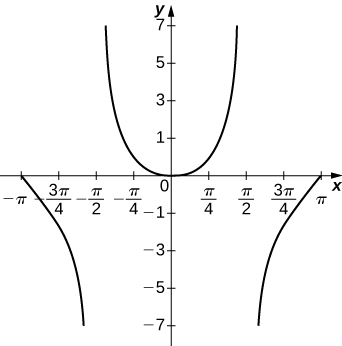
52. ![y=x \tan x,x=\left[\text{−}\pi ,\pi \right]](https://opentextbc.ca/calculusv1openstax/wp-content/ql-cache/quicklatex.com-1e0148e32992fb051fe44ec8189f7fcd_l3.png "Rendered by QuickLaTeX.com")
Solution
53. 
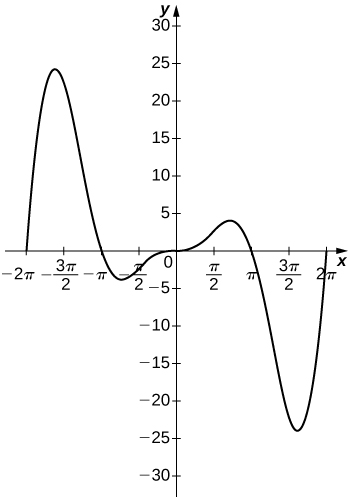
54. ![y={x}^{2} \sin (x),x=\left[-2\pi ,2\pi \right]](https://opentextbc.ca/calculusv1openstax/wp-content/ql-cache/quicklatex.com-a1a25dadd41f574a598047bc89665848_l3.png "Rendered by QuickLaTeX.com")
Solution
59. Truthful or false: Every ratio of polynomials has vertical asymptotes.

Source: https://opentextbc.ca/calculusv1openstax/chapter/limits-at-infinity-and-asymptotes/
Posted by: gordonhatelve.blogspot.com
0 Response to "How To Draw The Derivative Of A Rational Function"
Post a Comment